Set of Tools for successful Time Series Analysis
Stack of basic statistical tools you need for technical analysis of time series data
Intro 📈
This time I decided to write a post about common best practices I’m typically watching when analyzing time series data. These methods are quite widely known & used in the field of mathematics and statistics. I won’t go deeply into mathematical motivation behind patterns to keep things simple.
All-together, in my technical advisory work I’m dealing with plethora of different industries ranging from financial field to healthcare to sports. Today, almost every business-related process generates data. This opens completely new possibilities when data analytics & science can be leveraged for this work to generate new ideas.
Why time series data is one of the most common type ?🔥
Time series data can be found literally everywhere around us. Typically it’s generated as a result of multitude various processes like access management & devices like paper machines, elevators, healthcare devices, data centers, refrigerators. Common for all of them is the fact of running on 24/7/365 basis - and the data is generated as well up to real-time. This data type is well applicable on predicting such use cases like need for maintenance, optimizing processes or supply chains to changes in weather or understanding which variables have effect on product price trend formation.
Need for such operative data decomposition is real because of existing outliers, impreciseness and other factors which may have affect on the overall outcome.
Anyway, list of methods listed below isn’t exhaustive but sufficient to cover majority of needs to understand the data better & make predictions more precise.
Trend, seasonality and stationarity of data 🤖
Trend and seasonality is something we can observe in the data over longer period of time.
Stationarity (or non-stationarity) on the other hand describes whether observed data has zero mean & variance (for stationary data). Basically this assumes no trend in data. Otherwise, if this isn’t the case, certain behaviours like growing demand or trend over time may affect our prediction quality significantly (non-stationary data). Taking into account both these two types helps us to understand how to interpret the prediction outcomes.
Stationarity of data can be evaluated using Dickey-Fuller statistical method.
Finally, when these three aforementioned evaluations are inspected, I typically like to decompose (i.e. separate) trend, seasonality & stationarity into separate datasets to visualize patterns to understand data further.
It’s good to notice that it’s in most cases it’s prerequisite to remove trend & seasonality (i.e transform data from non-stationary to stationary) for prediction modelling but we won’t discuss it within’ this post.
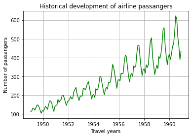
Example of trend:
We can observe growing trend of more flight customers or demand for product. This can happen, for instance, over period of 10 years. From figure above we can see year-over-year grow trend-pattern.
Example of seasonality:
Demand for specific type of apples in grocery store is seasonal because this particular type of apples is harvested around September. Another example can be amount of flights taken to a specific holiday destination because of the good weather conditions, let’s say, around November-December.
So, demand for specific product or time of year can trigger seasonality in behaviour and thus result seasonality pattern in data. From figure above we can notice clear seasonality-pattern as well.
Example of stationarity:
Case for stationarity can be found in price of highly standardised product which may fluctuate (variance) on occasion but over period of time stays about the same.
Example of non-stationarity:
Case for non-stationary data could be S&P 500 stock index with its’ unexpected fluctuations. It’s also good to notice that majority of data is typically non-stationary because of their nature.
When it comes to stationarity, above figure is example of non-stationary data since it shows that variance and mean are not constant.
Decomposition example:
Decomposition can be observed from figures below where with the help of functions trend and seasonality are separated as purely own time series data charts.
So there you have it - three simple statistical tools to leverage your time series data analysis which I utilize myself in my daily practice and are suitable for majority of use cases. 🙂
Now, I would like to hear from you, dear reader, which analytical methods do you prefer for conducting your time series/data analysis work? Which work for you, which don’t?
Additionally, are there topic suggestions you would me to cover in the future?
Hit a comment-button below 😎
Also, if you like what you have red, consider subscribing - it’s free and delivered straight to your mailbox 📫


